Or: Birding in the era of climate change

In my previous job as a researcher, I modeled hydrology of wetlands, including the playa lakes region. Visiting Kansas this weekend was my first time getting to spend time in that region since that project concluded, but sadly, I got to see the phenomenon we were testing: what drought on the landscape looks like. So, I embarked on a quest to find water with tools that are by and large accessible to birders.

I continue my evangelism of Google Earth Engine, which has somewhat quietly changed the game of remote sensing, though maybe more loudly in today’s research landscape: I was an early adopter when it first came out and swooned over the potential. Now, I imagine it has become a much more popular research tool, but I want the floodgates to open for hobbyists too. It is a truly remarkable game changer and uprooted how we always did things (e.g. during my PhD) to process and analyze remote sensing (e.g. satellite imagery) data. These days, you can pull from a library of images straight into your coding environment and mapping output (I still get goosebumps typing that). You can query a compendium of publicly available satellite images, write your code to analyze it, and display the output in one browser tab…oh, and did I mention the excellent documentation and gobs of available coding examples?

The Quarry

On this mission, I was specifically looking for Clark’s grebe (Aechmophorus clarkii): though their habitat requirements are flexible in migration, they tend to like big wetlands or lakes with deep, persistent water. These proclivities governed what I was able to do to identify suitable water bodies.

The Solution

I devised a script (below) to leverage Sentinel imagery to calculate normalized difference water index (NDWI) which is a well-known indicator of water on the landscape. You can copy the whole script right into your code editor and run it as-is, but I’ll walk through in general what it does in the remainder of the post. I also co-opted a fair number of code chunks from the Google Earth Engine examples, so you’ll find some of these functions (e.g. the cloud mask function) elsewhere in their documentation. I commented out some map layers as well, but you can play with adding them back in.

Methodology

First, I filtered the imagery down to the state of Kansas to make the analysis relevant and manageable. Given that playas are filled by rainwater and the problem was drought, I could be a little more focused in my image gathering: I looked at the 2 weeks prior to my arrival and kept images with < 30% cloud cover. (If you were looking at a rainier area or season, you would have to expand your time window and possibly adjust your cloud filter threshold to make cloudless composites of your area.) After masking out cloudy pixels, I calculated NDWI for each image (taken at a specific time and over a specific footprint).

I took the median over time for all the footprints to create one composite image. Of course, how you average and filter needs to be considered as you vary your time window: the longer your time window, the more possibility for e.g. a signal relevant to a given time period to be swamped out by conditions across the time span. I chose a threshold of only keeping pixels greater than or equal to 0.1 NDWI because this becomes fairly reliable for representing open water. I was also looking for a species that likes open and deeper water, so a conservative threshold represented suitable water bodies.

There’s an optional resource in this example that needs to be requested if you want to use it (i.e. is not freely downloadable): spatial range map files for birds of the world. If your data request is approved, you can pull out the files for your species of interest. I uploaded the shape file for my species of interest as an asset (clark) and imported it into my script by clicking the arrow that appears when you hover over it in the Assets tab. I just used it to display the range boundaries on the map. I commented out all of those lines in the script below, so if you don’t have a range map shape file (i.e. a polygon) to put in its place, just keep the script below as is:

var table = ee.FeatureCollection("TIGER/2018/States"),
    //clark = ee.FeatureCollection("users/gorzo/clark"),
    Sentinel = ee.ImageCollection("COPERNICUS/S2_HARMONIZED");

/**
 * Function to mask clouds using the Sentinel-2 QA band
 * @param {ee.Image} image Sentinel-2 image
 * @return {ee.Image} cloud masked Sentinel-2 image
 */
function maskS2clouds(image) {
  var qa = image.select('QA60');

  // Bits 10 and 11 are clouds and cirrus, respectively.
  var cloudBitMask = 1 << 10;
  var cirrusBitMask = 1 << 11;

  // Both flags should be set to zero, indicating clear conditions.
  var mask = qa.bitwiseAnd(cloudBitMask).eq(0)
      .and(qa.bitwiseAnd(cirrusBitMask).eq(0));

  return image.updateMask(mask).divide(10000);
}
                  
var spring2023 = spatialFiltered.filterDate('2023-04-01','2023-04-15')
                  // Pre-filter to get less cloudy granules.
                  .filter(ee.Filter.lt('CLOUDY_PIXEL_PERCENTAGE', 30))
                  .map(maskS2clouds);

var rgbVis = {
  min: 0.0,
  max: 0.3,
  bands: ['B4', 'B3', 'B2'],
};

/* Map.addLayer(spring2023.median(), rgbVis, 'RGB');
var empty = ee.Image().byte();
var outline = empty.paint({
  featureCollection: clark,
  color: 1,
  width: 3
});
Map.addLayer(outline, {palette: 'purple'}, 'AOI'); */

// Function to calculate and add an NDWI band
var addNDWI = function(image) {
return image.addBands(image.normalizedDifference(['B3', 'B8']));
};

// Add NDWI band to image collection
var spring2023 = spring2023.map(addNDWI);

var pre_NDWI = spring2023.select(['nd'],['NDWI']);
var NDWImg = pre_NDWI.median();
var ndwiMasked = NDWImg.gte(0.1);

ndwiMasked = ndwiMasked.updateMask(ndwiMasked.neq(0));

var vectors = ndwiMasked.reduceToVectors({
  geometry: ks,
  crs: NDWImg.projection(),
  scale: 234,
  geometryType: 'centroid',
  eightConnected: true,
});
Map.addLayer(ndwiMasked, {palette:['ff0000']});
Map.addLayer(vectors);

/*Export.table.toDrive({
  collection: vectors,
  description:'water_pts',
  fileFormat: 'KML'
});*/

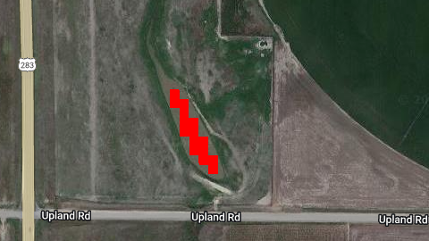
In the example map visualization left in the code, water bodies identified by this analysis are in red, which helped me pick them out as I was poring over my laptop in power saving screen mode on the go (yes, I was fiddling with this on the plane…and Southwest Wi-Fi had enough juice for me to play!). So, how do you then find these in the real world, assuming you don’t have your laptop propped on the dashboard of your rental car (I would never…)? I turned my raster layer (i.e. grid data, in this case the pixels of an image) into a vector layer (commonly known as shapes). The vectors variable in the code block is the output of a function that connects those water pixels into features by an 8 neighbor rule, and in this case, outputs the geographic centers of those features. At the end of the script, I commented the code out to save a KML of those points to your Google drive, but you could export them into a variety of formats. From there, you can get creative with optimizing a route between them (maybe that will yet be the subject of a later post).

Herein lies a bit of a limitation: that’s a costly operation, so you can only run something like that at a given scale, and in my case I found the magic number to be 166. So, features below that size are not identified (zoom into the map to see red water bodies not marked by a corresponding dot). That was sort of OK with me though, because the species I was looking for likes bigger water bodies. It would be limiting for looking for smaller wetlands though.

So how did it go? Sadly in all of my trip prep, I started this endeavor a little late and had to dust off the cobwebs in transit. I ended up trading off some geek out time for exploration. But, here was an intriguing looking wetland I found on the output image, and stopped at on my way back (for what it’s worth, too small to earn a point on the statewide version of the analysis I ran).

Maybe in keeping with the small size, no Clark’s grebes (though their stopover habitat requirements are much more flexible in migration) but plenty of cool waterfowl piled up at this little wetland. Now, armed with some tools locked and loaded, I’m ready for my next trip out west!

In this example, I had a shape file I wanted to use as a mask. However, the features were those I wanted to keep. In other words, I wanted to keep all the pixels that had values (i.e. not “no data”) that intersected with the shapes, and set those outside the shapes to 0. Then, I needed to set the no data value to 0, and only keep “clumps” of pixels w/values that were 88 or more.

gdal_rasterize -i -burn 0 mask.shp input.tif
gdal_translate -a_nodata 0 input.tif output.tif
gdal_sieve.py -st 88 -8 output.tif

Voila! (The mask can also be a geo package, with the layer specified using the -l option.)

ogr2ogr output_dissolved.shp forest_VGS.shp -dialect sqlite -sql “SELECT ST_Union(geometry) AS geometry FROM forest_VGS”